RM

Long queuing times and overcrowding in school cafeterias are known to be serious problems faced by students.
This issue has been well-documented in previous studies that have emphasized the impact of poorly designed cafeterias on student satisfaction, waiting times, and the overall dining experience. Surveys conducted at our school have shown that many students are dissatisfied with the current cafeteria setup, citing overcrowding and long wait times as major annoyances.
However, no one has fully explored why these issues persist after years of improvement, or how specific factors - such as cafeteria layout, queuing systems, and crowding during peak hours - contribute to the problem.
If we can identify the root causes of inefficient cafeteria operations, we can not only improve the dining experience, but also optimize space usage and human resources.
This study aims to investigate the root causes of cafeteria crowding by analyzing queuing dynamics, conducting simulations, and exploring potential improvements. By identifying and addressing these issues, we hope to reduce queue times, increase student satisfaction, and improve overall operational efficiency.

DataCollection

Observation

The data for this study came from field observations in the our school’s cafeteria, and data were collected from December 2 to December 5, 2024 and December 9 to December 12, 2024 (8 days in total). Data collection under each schedule lasted for four days due to the school’s schedule of one cycle every two days. The data primarily covered the third and fourth period that are lunch periods, the peak hours. Specifically, it includes the number of students enter/leave the cafeteria during each period, the service time of each window, and the number of windows.

Methodology

Data collection was performed through the cafeteria’s monitoring system during the daytime hours, which recorded the timestamp of each student’s entry into the cafeteria. The specific time period for data collection was from 11:50 to 13:35 each day.During this time period, the number of students entering the cafeteria was recorded by manual count and the service time of each service window was recorded by simple observations. The mean value of the window service time is the average value obtained by several manual timings.

Data preprocessing

During the data cleaning process, all the collected data met the preset criteria, so no data was eliminated. During the data preprocessing stage, timestamps were converted to relative times with respect to peak hours and grouped for counting at 2-minute intervals during peak hours. For off-peak hours, group counts were performed at 5-minute intervals.

Data characterization

The results of the data analysis showed that the arrival time of students to the cafeteria showed obvious peak characteristics, especially between 11:50 and 12:10, when an average of about 40 people entered the cafeteria per minute, while the number of arrivals decreased significantly at other times. The distribution of service times at the service window roughly conforms to an exponential distribution and has an average service time of 45 seconds. Detailed statistics have been presented in Figure X.

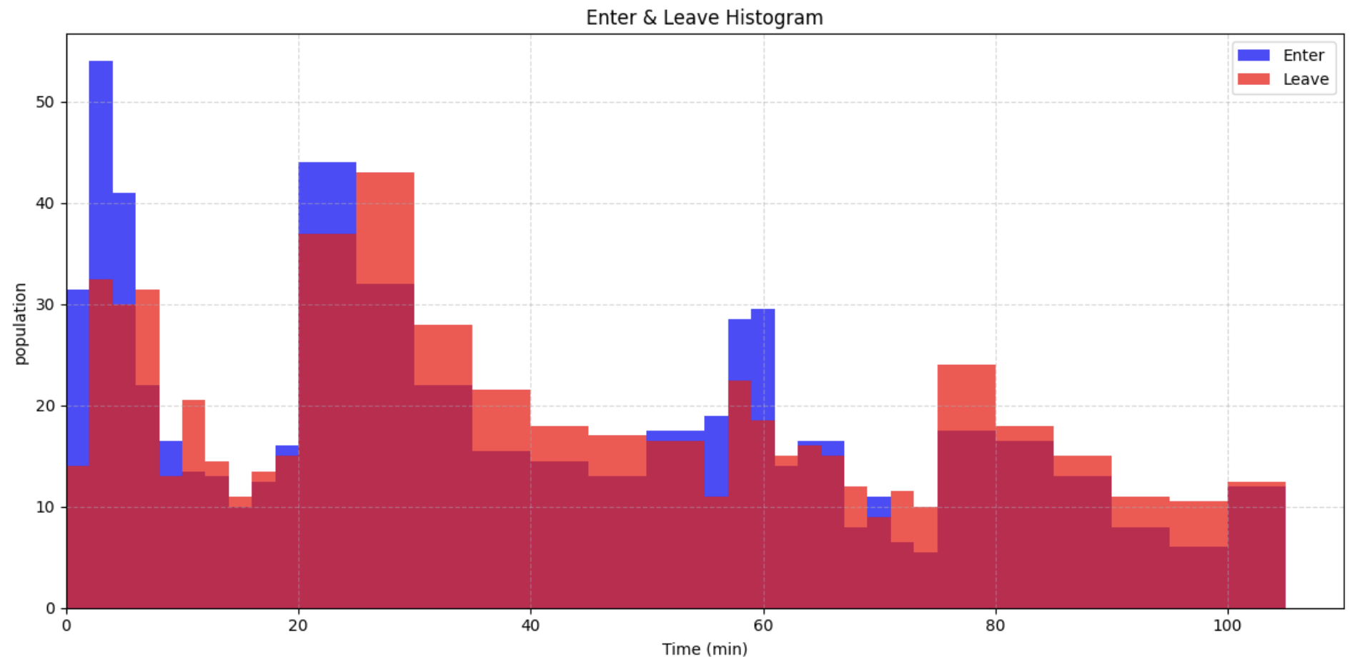
[Figure X … Description]

We can also graph the net population in the cafeteria.

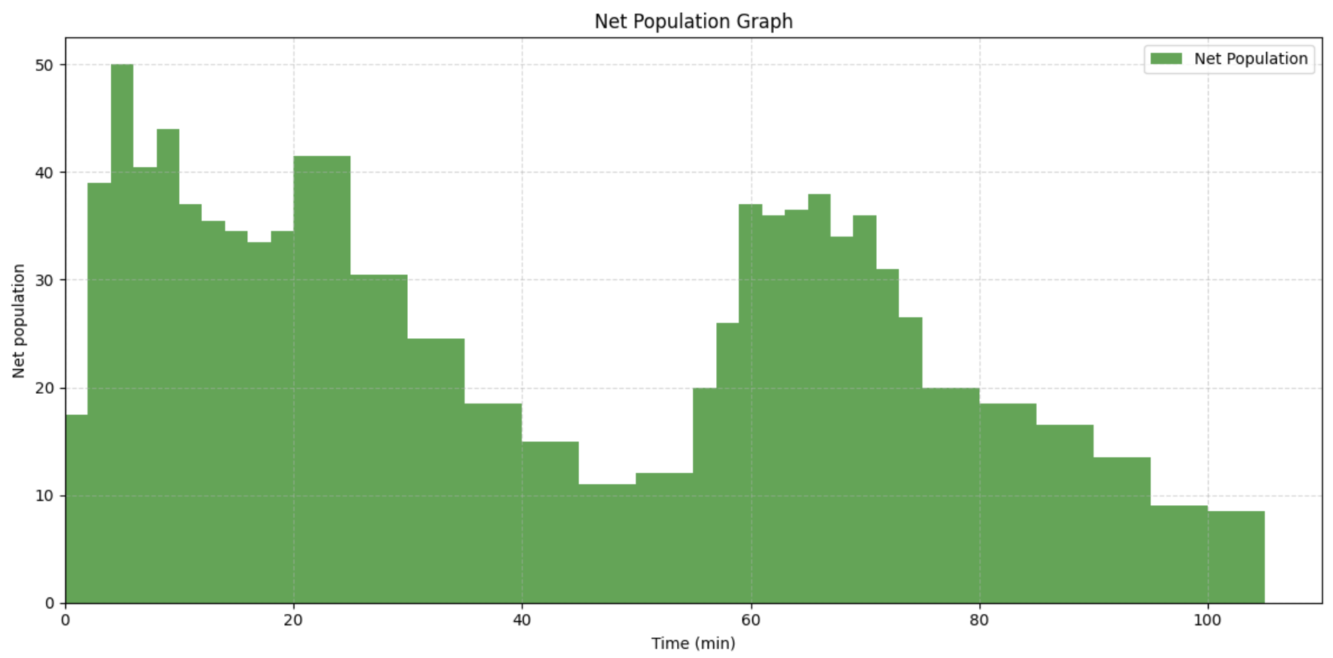
[Figure X … Description]

Similarly, there are particularly large numbers of students at the start of the P3 and P4, and then the numbers drop off over time.

Data Processing

Once the data collection was complete we next used the data to calculate the student arrival rate, which is a variable that changes over time during every lunch time.

Symbol	Description	Unit
$E_t$	Total number of individuals entering the location during interval t	Count
$L_t$	Total number of individuals leaving the location during interval t	Count
$p_{pass}(t)$	Probability that an entering individual is passing through	Fraction
$p_{service}(t)$	Probability that an entering individual seeks service	Fraction
$q_{leave}(t)$	Probability that a service seeker leaves immediately after service	Fraction
$r_{stay}(t)$	Probability that a service seeker stays after service	Fraction
$S_t$	Number of individuals arriving for service during interval t	Count

Total Population

We get the average Entries and Exits ($E_t$ and $L_t$) by simply adding them together and divided by the number of days. Notice that our school’s cafeteria has 2 entrances (marked as A and B here).
So for each time interval t:

$$Tota{l}_{Enter}=\frac{{\text{Enter A}}_{Day1}+{\text{Enter A}}_{Day2}+\text{...}+{\text{Enter A}}_{Day8}}{8}+\frac{{\text{Enter B}}_{Day1}+{\text{Enter B}}_{Day2}+\text{...}+{\text{Enter B}}_{Day8}}{8}$$

It is the same way to calculate $Tota{l}_{Leave}$

Number of Service Seekers Arriving During Interval t ($S_t$)

Then we consider the following factors. We know that not all of the students who enter the cafeteria will have any food, and that some may only stay for a short time before leaving (e.g., using the cafeteria as a hallway just to walk through it). In addition to this, since our school has an outdoor dining area. It has the same capacity as an indoor cafeteria. Some people order their lunch and go straightly to the outdoor dining area, while others stay indoors to eat their lunch. We will mainly focus on those students who stay indoors.

We have a fraction $p_{service}$ of entrants seek service, where $p_{service}(t)$ = $1-p_{pass}(t)$. Some service seekers leave immediately ($q_{leave}$), and some stay after service ($r_{stay}$) where $r_{stay}=1-q_{leave}$. However, $q_{leave}(t)$ does not vary roughly with the time in a day, but it has been observed that it increases significantly during the cold season, when people are reluctant to have lunch outdoors where it is colder. So in winter it usually gets more crowded indoors.

Assuming that the number of people leaving ($L_t$) corresponds to those who sought service and then left immediately, we can model:

$$L_t=q_{leave}(t)\times S_t+E_t\times p_{pass}(t)$$

Therefore, the number of service seekers arriving during interval t is:

$$S_t=\frac{L_t-E_t\times p_{pass}(t)}{q_{leave}(t)}$$

We can also get the individuals who stay after receiving service although we don’t mainly focus on it here:

$$R_t=r_{stay}(t)\times S_t$$

Using the above formula we calculated the arrival rate of students at different time periods, as shown in the figure (the code is buggy the figure is not generated yet, add it later).

I tried to fit the data set to a function, given its multi-peaked characteristic I decided to use a polynomial function. Starting with a $1^{st}$ order polynomial I gradually increased the order and calculated the $R^2$ value for each fit, I ended up with an $R^2$ value of about $0.92$ on the $8^{th}$ try, which I then recorded as being largely adequate for the needs of the study. The fitted function is shown below. (The graph also has many bug such as the wrong title and rough curve. I will fix it in the latest version)

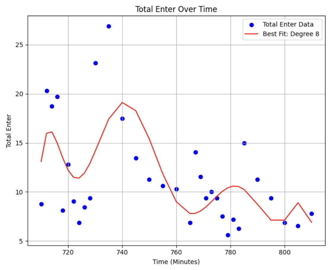
[Graph x, …description]

Model Establishment

Based on assumptions about the data and usual observations, we assume that the arrival distribution satisfies a certain distribution (e.g., skewed distribution). Most students usually enter the cafeteria right after classes end, and the arrival rate of people decreases steadly over time. We assume that the service process is a poisson process, i.e., each service time is completely random (not depend on any previous situation).

So the $G/M/c$ model should be used. (Note: the actual model selection needs to be based on actual data)

In the $G/M/c$ model, the arrival process follows a General distribution, the service time follows a Poisson process, and there are $c$ parallel service windows.

Basic Parameters

Symbol	Explanation	Unit
$\lambda$	Average arrival rate of customers	$people/s$
$\mu$	Average service rate of a single service window	$services/s$
$c$	Number of service windows	$Number$
$\rho$	system utilization rate	$/$
$C_a$	Coefficient of variation	$/$
$W_q$	Mean Waiting Time	$s$
$L_q$	Average number of people in the queue	$Number$
$P_0$	Probability that the system is empty	$/$
Which:

$$\rho =\frac{\lambda }{c\mu }$$

where $\rho <1$ is necessary for system stability.
$C_a$: coefficient of variation (ratio of standard deviation to mean) of the arrival time distribution:

$$C_a=\frac{{\sigma }_a}{1/\lambda }$$

Standard deviation of arrival times ${\sigma }_a$, We have a Set of data $[T_{a1},T_{a2},\dots ,T_{an}]$，We can estimate ${\sigma }_a$ by：

$${\sigma }_a=\sqrt{\frac{1}{n-1}\sum _{i=1}^n{\left(T_{ai}-\overline{T_a}\right)}^2}$$

$\overline{T_a}=\frac{1}{n}{\sum }_{i=1}^n{T}_{ai}$ is the average of arrival times
Mean Waiting Time $W_q$, Using a generalized form of the Pollaczek-Khinchin (P-K) formula, you can compute the average wait time in the queue $W_q$:

$$W_q=\frac{C_a^2+1}{2}\cdot W_{q,M/M/c}$$

where $W_{q,M/M/c}$ is the average waiting time of the $M/M/c$ model, Eq:

$$W_{q,M/M/c}=\frac{L_{q,M/M/c}}{\lambda }$$

Average number of people in the queue $L_q$
And $L_{q,M/M/c}$ (the average number of people in the queue) is based on the Erlang-C formula:

$$L_{q,M/M/c}=\frac{P_0\cdot \frac{(\lambda /\mu {)}^c}{c!}\cdot \frac{c\rho }{(1-\rho {)}^2}}{\left({\sum }_{k=0}^{c-1}\frac{(\lambda /\mu {)}^k}{k!}\right)+\frac{(\lambda /\mu {)}^c}{c!}\cdot \frac{1}{1-\rho }}$$

Revised $L_q$ is defined by：

$$L_q\approx \frac{C_a^2+1}{2}\cdot L_{q,M/M/c}$$

Probability that the system is empty $P_0$
$P_0$: the probability that the system is empty, which can be calculated by the following formula:

$$P_0={\left(\sum _{k=0}^{c-1}\frac{(\lambda /\mu {)}^k}{k!}+\frac{(\lambda /\mu {)}^c}{c!}\cdot \frac{1}{1-\rho }\right)}^{-1}$$

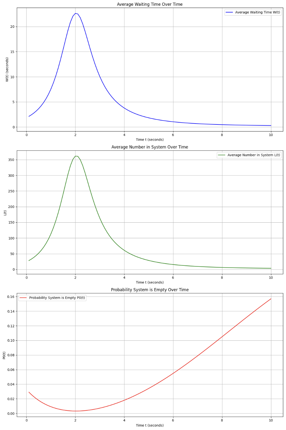
Average system wait time $W$
The average wait time in the system $W$ includes the wait time in the queue $W_q$ and the service time:

$$W=W_q+\frac{1}{\mu }$$

Average number of people in the system $L$
The average number of people in the system $L$ includes the number of people in the queue $L_q$ and the number of people being served:

$$L=L_q+\frac{\lambda }{\mu }$$

The result is graphed below: (Big problem, to be modified)

3. Model Using

FootNote

Use $C_a$ (Coefficient of Variation of Arrival Time) to correct the formula of $M/M/c$, that is, we can get the result of $G/M/c$.

Outputs

• We enter the observed data into the code segment and conclude that

The average arrival time is…
The average number of people in the queue is…

Extra

• Enhanced parameter estimation methods: Currently, parameter estimation is mainly based on best fit, but a more rigorous calculation of confidence intervals should be incorporated.
  • Calculate confidence intervals for parameter estimates using the Bootstrapping method.
  • Check the stability of the estimates by estimating them separately for different time periods and